Reference

Exhaustive description of the InTerra Studio interface and every tab.

The interface

The parts of InTerra Studio that aren't tied to a single tab: the window layout and map gestures, the Start Window, the menus, and the notification center.

The map-and-panel layout

Most tabs share the same shape: a controls panel on the left and a map on the right. The left panel is where you make choices and read values; the map shows your site, flight, footprints, targets, and boundaries in context. The two stay in sync — selecting something in the panel highlights it on the map, and vice-versa.

Working with the map

The map panel behaves consistently across tabs, so the gestures you learn on one tab work everywhere:

• Pan by dragging, and zoom with the scroll wheel, to move around the site.
• Search to a place using the address box on Project Information to jump straight to your survey area instead of panning across the globe.
• Draw and edit the boundary on Project Information by placing vertices around your site; the boundary you draw is reused everywhere downstream.
• Drag interactive markers — for example, the datum marker on Target Planning — directly on the map to position them.
• Selection stays in sync — picking a photo, target, or point in the left-hand panel highlights it on the map, and selecting it on the map highlights it in the panel.

The basemap imagery is also what Suggest Colors (on Target Planning) samples to recommend high-contrast target colors for your specific ground.

The location gate

The very first thing InTerra needs to know is where your site is. Until you set a project location (on the Project Information tab), the other tabs are intentionally locked behind a gentle "set your location first" overlay. This is not a bug — almost everything downstream (footprints, GSD, coverage, ground control, map basemaps) depends on knowing the site's position, so InTerra asks for it up front.

The Start Window

The Start Window is the first thing you see when you launch InTerra Studio (its title bar reads InTerra Studio – Start). It is your home base for opening existing work or starting something new, and it carries the InTerra Studio branding and logo.

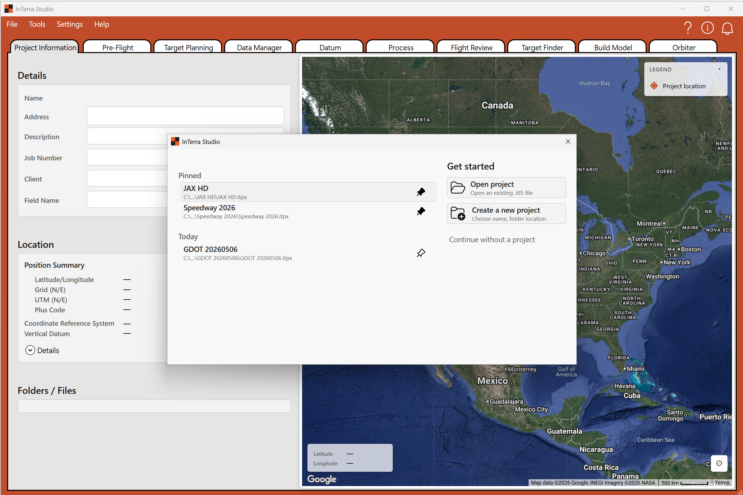
Screenshot: the full Start Window — the recent-projects list on the left and the Get Started panel (Open / Create) on the right, with the InTerra Studio logo visible.

• Recent Projects (left) — your projects, split into Pinned (jobs you've marked to keep at the top) and Older (everything else, most-recent first). Double-click to open; right-click for a context menu to Pin/Unpin, Remove from List (tidies the list without deleting from disk), or Copy Path (copies the project's folder path to your clipboard).
• Get Started (right) — Open project to browse for an existing project (handy when one isn't in the recent list, e.g. copied from another machine); Create a new project to start fresh (InTerra asks for a name and folder location, builds the project structure, and opens it ready to set the location); or Continue without a project to open the app without loading one.
• Reopening it — you don't have to restart the app. Any time you're in a project, choose File → Start Window… to bring it back, useful for hopping between jobs.

The main window and menu bar

Once a project is open you're in the main window: the menu bar and toolbar across the top, the tab strip beneath it, and the active tab filling the rest of the window.

Screenshot: the main window with a project open — the menu bar and toolbar icons across the top, the tab strip beneath, and a tab's content filling the window.

File — New Project (same as the Start Window's create); Load Project… (open from disk); Start Window… (bring back the Start Window without closing your project); Save Project (Ctrl+S — saves metadata, settings, ground-control picks, and choices into the project folder; get in the habit of pressing it after meaningful changes); Recent Projects (a submenu with inline pin/remove buttons); and Exit.

Tools — Coordinate Transformation…, a standalone calculator for converting coordinates between reference systems (useful when a client hands you a control point in one datum/projection and you need it in another); and SmarTarget® Manager…, which downloads the raw GNSS logs (.ubx) from your SmarTarget field units over USB (detailed under Locator tabs → SmarTarget Manager below).

Settings — Branding… opens the Settings window to control how your client-facing reports look: your company logo, identity details, and the report footer, with a live preview. Branding is set once and reused on every report, so a finished deliverable carries your company's identity rather than InTerra's. (See the report outputs under Modeler tabs → Build Model.)

Help — View Help opens this documentation; About shows the version, license key, license type, credit balance, and days remaining on the license.

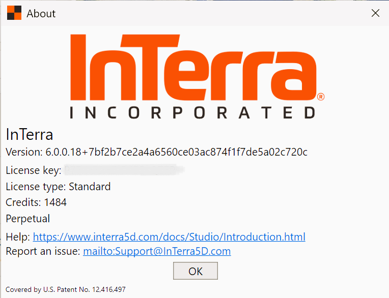
Screenshot: the About box showing the version, license type, credits, and days-remaining lines.

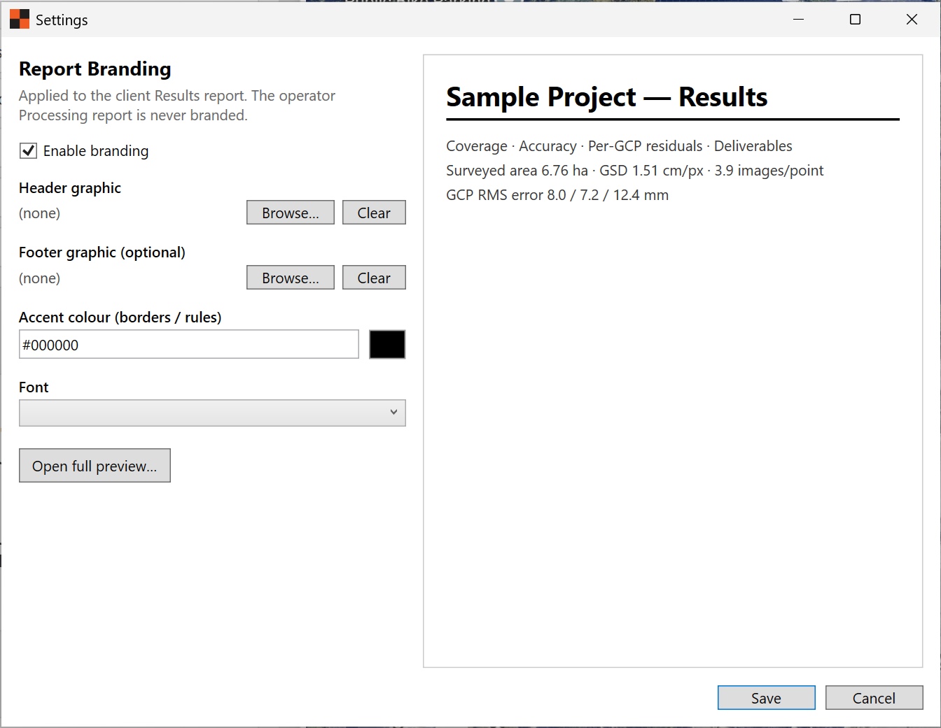
Screenshot: the Settings → Branding… window with a sample logo loaded and the live report preview visible.

Toolbar and notifications

Quick-access icons sit at the top-right: Help (opens this documentation), About (opens the About box), and the Notifications bell (opens the notification center).

The notification bell collects messages InTerra wants you to see without interrupting your work — license reminders (for example, "your license expires in N days"), cloud-processing status, and other updates. A badge tells you when something new has arrived. License messages in particular always surface here (and as a friendly dialog when important) rather than failing silently, so you're never caught off guard.

Locator tabs

The Locator module sets up the project, plans the flight and target layout, and turns your field GNSS logs into survey-grade ground control. Project Information establishes the site and coordinate system; Pre-Flight and Target Planning plan the mission before you fly; and SmarTarget Manager, Data Manager, Datum, and Process correct your SmarTargets (and the Datum) against a reference to produce ground control points.

Project Information

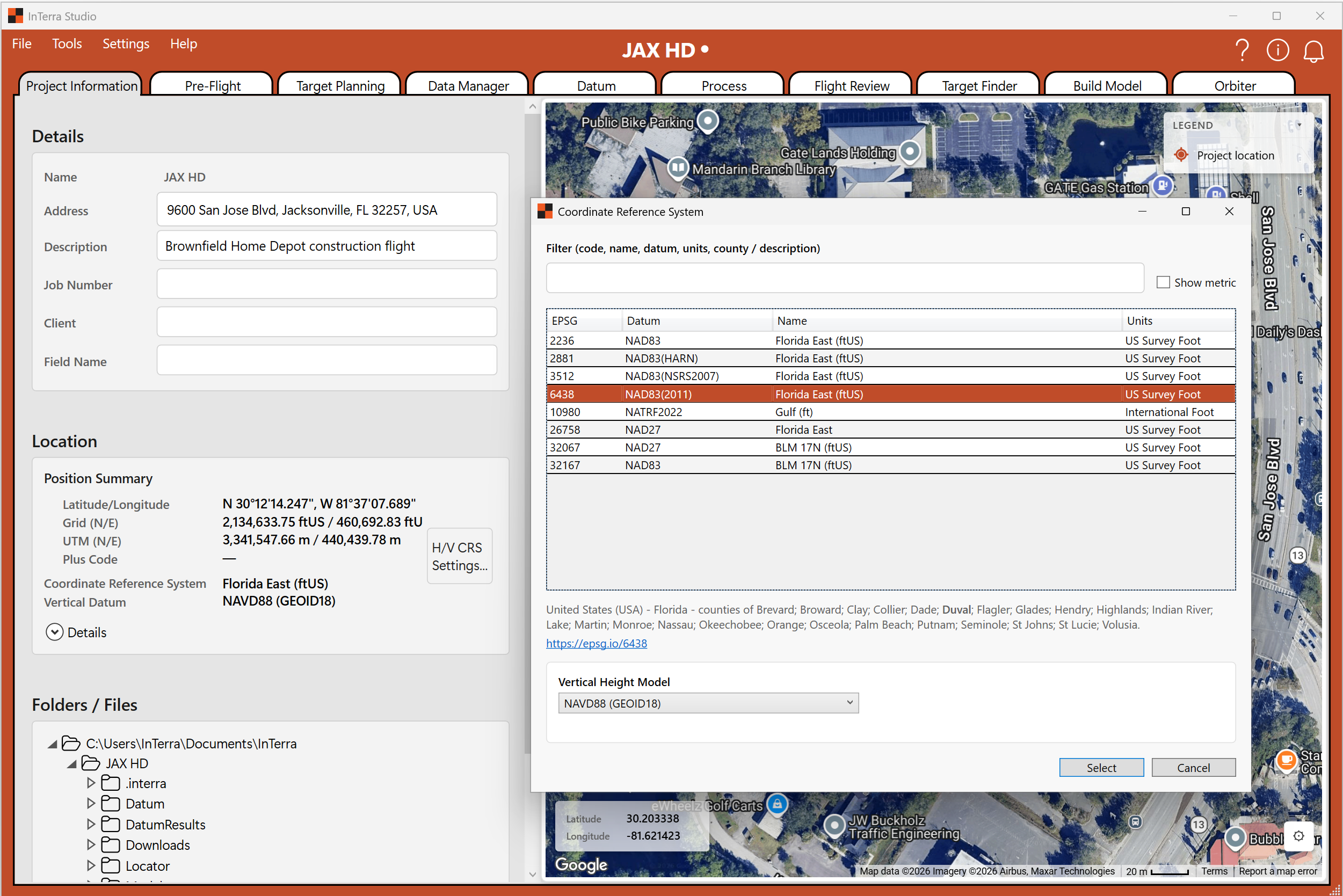
Screenshot: the Project Information tab with the site located and a boundary drawn — the Details, Location & Boundary, and Coordinate-system cards on the left, and the boundary polygon on the map.

What it's for. This is where a project begins: you give it an identity, pin it to a place on the earth, and choose the coordinate system your deliverables will use. Setting the location here is what unlocks the rest of the tabs.

When you use it. First, on every project — and any time you need to revisit the project's metadata, boundary, or coordinate system.

What you'll see. A controls panel on the left with three cards, and the map on the right.

• Details. The project's name, an address with a map search box (start typing an address or place and InTerra geocodes it to drop you on the site), and a free-text description. The name and address also flow into your client-facing report header, so it's worth filling them in cleanly.
• Location & Boundary. Place the site on the map and draw the area boundary — the polygon that describes your project's extent. The boundary does real work later: it defines the area InTerra models, drives coverage statistics, and can clip your deliverables to just the site (see Modeler tabs → Build Model). Take a moment to draw it accurately.
• Coordinate system (CRS). Choose the reference system your project works in and whether heights are ellipsoidal or orthometric. You usually don't have to choose blind: once you set the location, InTerra picks sensible defaults for you — both the horizontal system and the heights. In the US it defaults to the State Plane zone for the site's county (in feet, on the latest NAD83 realization) with orthometric heights on GEOID18; UK and other regions follow their own national-grid rules. When the location is ambiguous (a county that straddles two zones, say), InTerra opens the CRS picker so you can confirm. You can always override the defaults — if your client specified a particular state-plane zone, a UTM zone, or a specific vertical datum, set it here. This is the single most important setup choice for survey accuracy: it determines the frame your orthophoto, elevation models, and point cloud come out in.
• File Explorer. Browse the project's folder tree right inside InTerra, so you can see what files exist and where deliverables land without leaving the app.

Tips.

• Set the location and boundary first — the location gate on other tabs is waiting on it.
• Get the coordinate system right early. Changing it after you've done a lot of downstream work means re-checking anything that depended on it.
• Set the address first and let the CRS default. Because the coordinate system is chosen from the location, entering the site address before you touch the CRS card usually lands you on the right horizontal system and orthometric heights (GEOID18 in the US) automatically — you only need to touch the card if your client wants something different.
• Use the address search to jump to the site quickly instead of panning the map around the world.

Pre-Flight

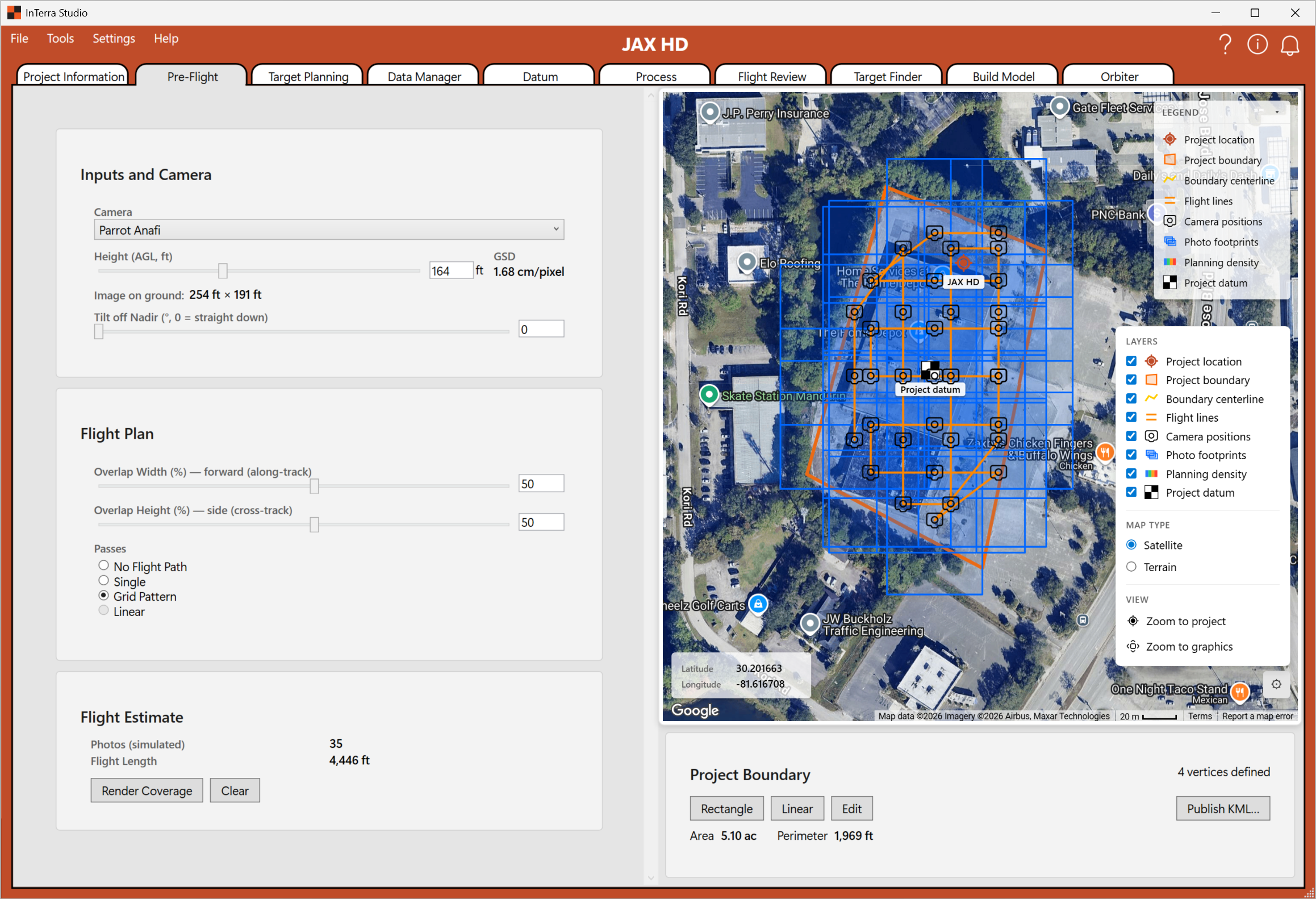
Screenshot: the Pre-Flight tab with a camera selected and a height set, showing the GSD readout in the left panel and the single-photo footprint drawn on the map.

What it's for. Work out the relationship between your camera, your flight height, and the resolution and footprint you'll capture — so you can pick a height that hits your target ground sample distance (GSD).

When you use it. While planning a mission, before you fly.

What you'll see. An Inputs & Camera card on the left and the map on the right.

• Camera. Choose your camera from a dropdown. InTerra uses the camera's sensor and lens characteristics to compute footprint and resolution.
• Height (AGL). Set your planned height above ground level with a slider and a numeric box. The control is units-aware (steps by 1 m or 5 ft).
• GSD readout. As you change camera and height, InTerra shows the resulting ground sample distance — the real-world size of one pixel on the ground. Lower GSD (e.g. 1.5 cm) means finer detail; it usually means flying lower and capturing more photos.
• Ground footprint. The area a single photo covers on the ground at your chosen height, so you can reason about overlap and coverage.
• Nadir / tilt. The camera-angle assumption used in the footprint geometry (typically straight down, "nadir").

Tips.

• Decide your required GSD first (often dictated by the deliverable's accuracy spec), then use the height slider to find the AGL that produces it.
• Remember that lower height = finer GSD = more photos = longer processing. Pre-Flight is where you make that trade-off deliberately instead of discovering it later.

Target Planning

Screenshot: the Target Planning tab after scattering targets — the targets on the map and the target grid (with color swatches) in the left panel.

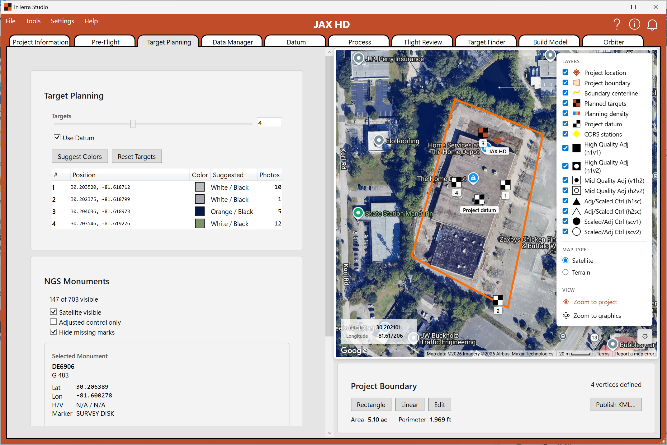
Screenshot: (optional detail) the result of Suggest Colors, showing the recommended high-contrast scheme.

What it's for. Decide how many ground targets to place and roughly where, and choose target colors that will stand out in your imagery — so the markers are easy to find and tag later in Modeler tabs → Target Finder.

When you use it. During planning, alongside Pre-Flight — and to refine the target layout before heading out.

What you'll see. A Target Planning card on the left and the map on the right.

• Targets slider. Choose how many targets to scatter across your site (0–10). InTerra distributes them across the boundary as a starting layout you can adjust.
• Use Datum. Turn on a datum marker — a reference point seeded from the boundary's center that you can drag on the map to where you'll set your base or reference position.
• Suggest Colors. InTerra samples the basemap imagery of your site and recommends high-contrast color schemes (for example, orange/black or white/black) so your physical targets pop against the ground in the photos. Good contrast here saves real time when you're tagging control points later.
• Reset Targets. Re-scatter the same number of targets to a fresh layout.
• Target grid. A compact table of your planned targets: index number, position (latitude, longitude), a color swatch, and the scheme name.

Tips.

• Spread targets toward the edges and corners of the site, not just the middle — good geometry improves the accuracy of the georeferenced model.
• Use Suggest Colors before you buy or paint targets; a scheme that contrasts with your specific site (grass, asphalt, dirt) is far easier to detect than a generic choice.

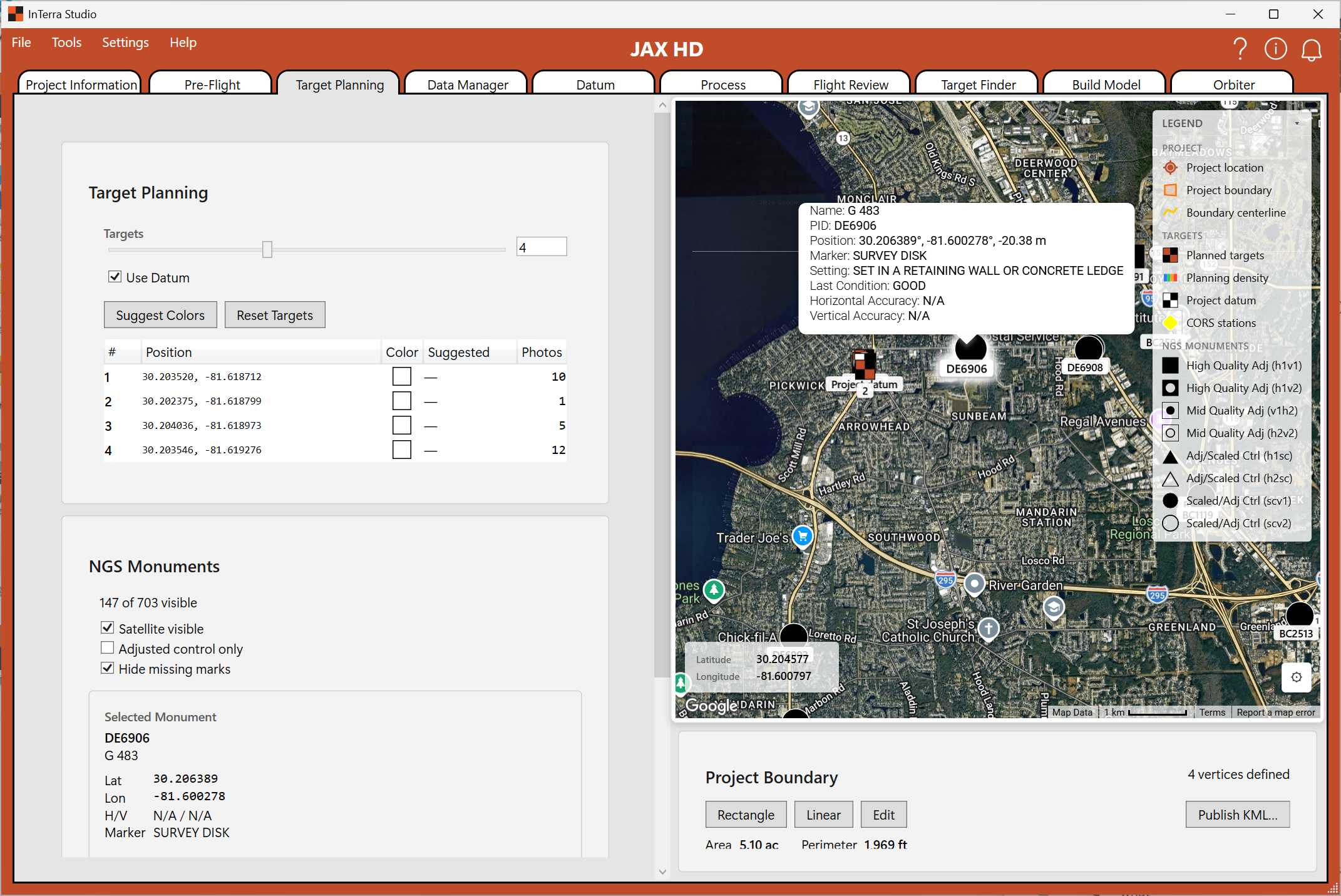
NGS monuments overlay (US only)

Once your project location is set, Studio queries the NOAA NGS geodetic-control monument shapefile for the project's state and shows every monument within ~10 km of the site on the map. These are surveyed reference points the federal government maintains — a free local source of high-quality control you can tie your project to (or use as an independent check on your own results).

Each monument's marker shape encodes what kind of control it provides (horizontal, vertical, or both) and how well-adjusted it is. The legend shows all eight types; prioritise them in this order:

Marker	Code	What it means	Use it for
Filled square	H1V1	Adjusted horizontal + adjusted vertical	Best 3D control — first choice for a project basepoint
Filled square + open inner circle	H1V2	Adjusted horizontal, other vertical	Strong horizontal, weaker vertical
Open square + filled inner circle	H2V1	Other horizontal, adjusted vertical	Strong vertical, weaker horizontal
Open square + open inner circle	H2V2	Other horizontal + other vertical	Acceptable reference, not a primary basepoint
Filled triangle	H1	Adjusted horizontal only	Horizontal reference where vertical isn't needed
Open triangle	H2	Other horizontal only	Less-reliable horizontal reference
Filled circle	V1	Adjusted vertical only	Vertical reference where horizontal isn't needed
Open circle	V2	Other vertical only	Less-reliable vertical reference

The general rule: filled shapes are adjusted control (the federal network has computed coordinates by adjusting them against the wider geodetic framework); open shapes are scaled or otherwise derived and should be treated as reference rather than primary control.

The remaining Locator tabs take the raw satellite-positioning data you recorded in the field and turn it into precise, corrected positions — the backbone of survey-grade accuracy. Your SmarTargets (and the InTerra Datum unit) are corrected against a base-station reference to produce ground control points; this processes your targets, not the drone's flight path. SmarTarget Manager gets the raw logs off your field units, then Data Manager, Datum, and Process turn them into corrected positions.

In the field? See SmarTarget in the field below for the hardware reference — LED meanings, the cloth targets, the field workflow, and battery / charging.

SmarTarget Manager

Opened from Tools → SmarTarget Manager… — a window, not a tab, but the first step in the GNSS workflow.

Screenshot: the SmarTarget Manager with connected units listed (number/Datum, battery, firmware) and their .ubx logs selected for download.

What it's for. Pull the raw GNSS logs (.ubx files) off your SmarTarget units. A SmarTarget is a GNSS logger that sits on a cloth ground target during the flight — so each one is both a visible ground control point and the device that recorded its own precise position. (The same hardware, set up as your InTerra Datum™ unit, can serve as the local base station that corrects the other targets.) Getting these logs off the hardware is the first step toward Ground Control Points: downstream, each .ubx is converted to RINEX (a standard GPS-data format) and corrected against a known reference — a CORS station, your InTerra Datum unit, or a local or restricted base station (such as a state DOT's) — to produce GCPs that lock the horizontal and vertical accuracy of the photogrammetry results. (Data Manager, Datum, and Process do that part; this tool just downloads the logs.)

When you use it. As soon as you're back from the field, before Data Manager — it's how the logs get from the hardware onto disk.

What you'll see. Every SmarTarget unit currently connected, a file table for the selected unit(s), and a download-folder picker.

• Connected units. Plug your units in over USB — a powered USB hub lets you connect and charge several at once. Each unit shows its number — 1–5 for the SmarTargets on your ground targets, or Datum for a unit set up as the InTerra Datum (base/reference) — along with its battery level and firmware version.
• Log files. A grid lists the unit's .ubx logs with size and capture date. Select the ones you want (multi-select works) and Download.
• Download folder. Choose where logs are saved. Files land named InTerra<unit>-<name>.ubx (e.g. InTerra3-… for target 3, InTerraDatum-… for the base), each with a per-file progress bar. Logs already in the folder are flagged so you don't pull them twice.
• Delete. Once a unit's logs are safely downloaded, remove them from the unit to free space for the next survey — select rows, then Del or right-click → Delete (you'll be asked to confirm).

Tips.

• Download every unit for the survey: the Datum unit anchors your corrections, and each numbered target needs its log for processing.
• Keep an eye on the battery column — a unit low on charge can drop mid-download.
• The downloaded .ubx files feed straight into Data Manager (which discovers them), then Datum and Process.

Data Manager

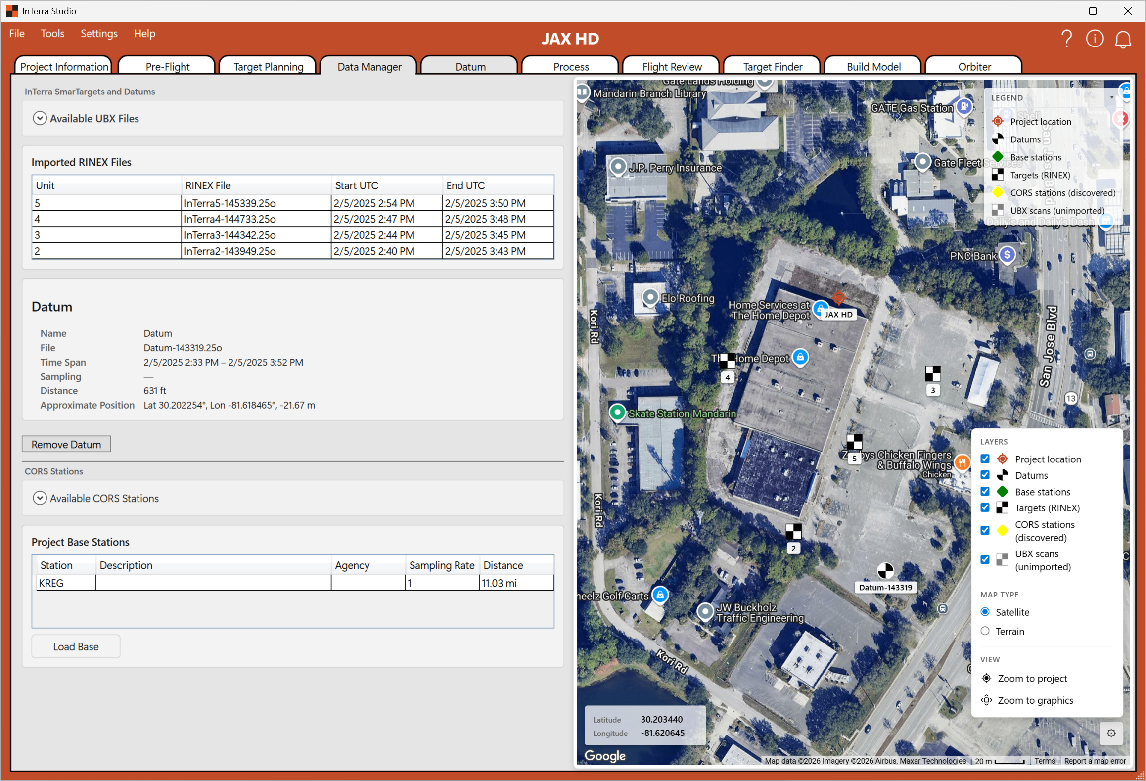
Screenshot: the Data Manager tab with discovered UBX files listed and selected for import, and the Base Station info card visible in the left panel.

What it's for. Bring your GNSS receiver logs into the project and manage the base-station data used for correction.

When you use it. Right after a survey, as the first step in GNSS processing — importing the logs off your receiver.

What you'll see. A controls panel on the left (file discovery and base-station information) and the map on the right.

• UBX file discovery. InTerra finds the UBX GNSS log files from your receiver. An Available UBX Files section lists what it found, with a settings button to tune how the scan works.
• Scan settings. A popup to adjust how InTerra discovers and interprets UBX files — useful when your files are organized in a particular way.
• UBX files grid. A short table of the discovered logs. Select the ones you want (you can multi-select) and import them into the project.
• Base Station info. A card summarizing the base-station data — what InTerra knows about the reference receiver that will anchor your corrections.

Tips.

• Import all the relevant logs for the survey window so later steps have complete coverage of the flight's time span.
• If files aren't showing up as expected, open scan settings and check the discovery options.

Datum

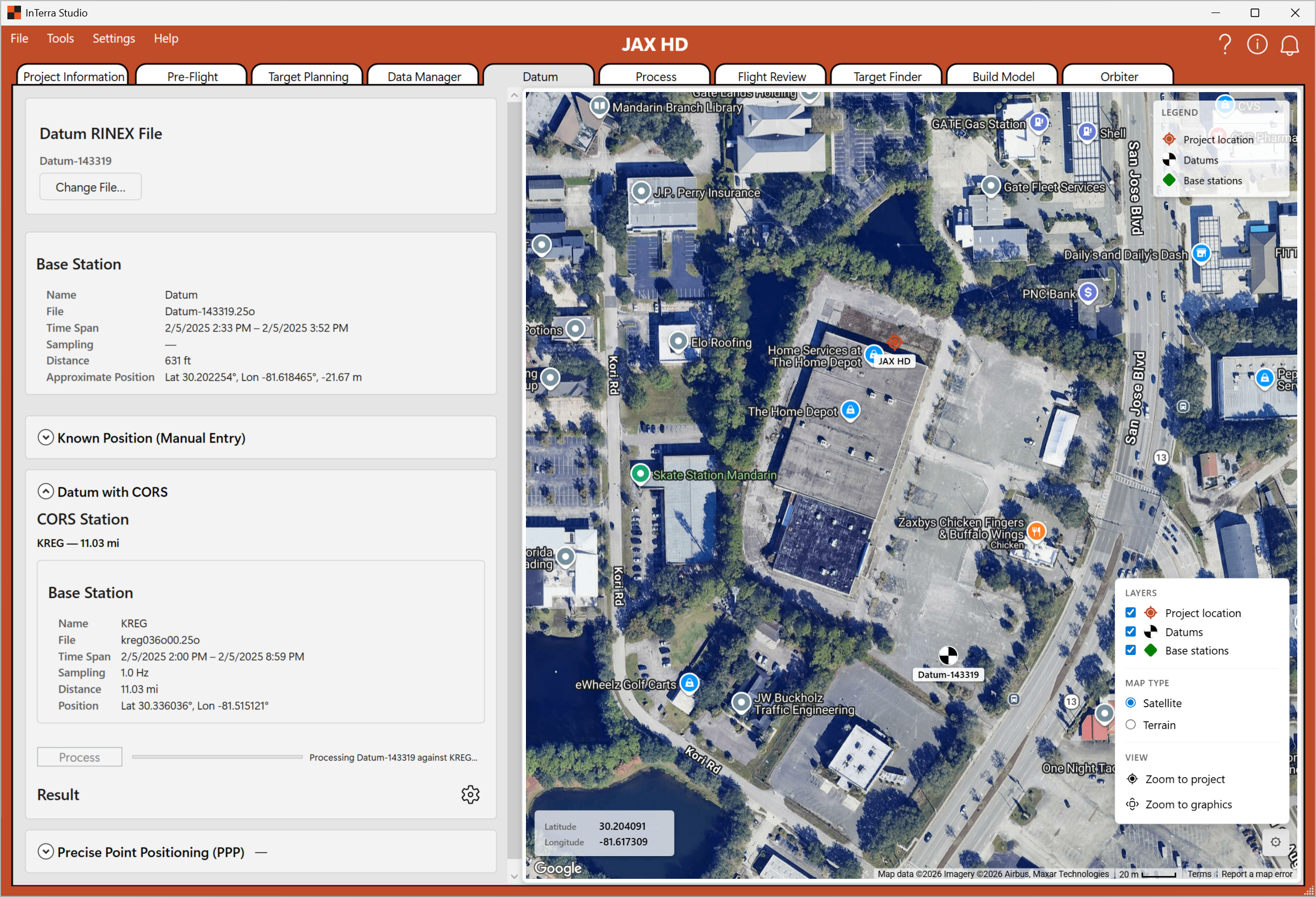
Screenshot: the Datum tab showing the selected datum RINEX file, the Base Station Info card, and the Known Position entry fields (latitude / longitude / altitude).

What it's for. Choose and configure the base-station (datum) reference your survey is measured against — the RINEX file (and its known position) that everything else is corrected relative to.

When you use it. After importing data, to lock in the reference position.

What you'll see. A controls panel on the left and the map on the right.

• Datum RINEX file. If there's a single datum it's shown as a filename; if you have two or more, you pick from a dropdown. Use Change File to point at a different RINEX file.
• Base Station Info. The shared base-station summary card, so you can confirm you've selected the right reference.
• Known Position. Enter the base station's known coordinates (latitude, longitude, altitude) when you have a surveyed position for it. Supplying a precise known position is what upgrades your whole survey from "relatively accurate" to "absolutely accurate."

Tips.

• If you only have the base's approximate (autonomous) position, your results are referenced to that approximate point. When absolute accuracy matters, enter a known position (or PPP-refine it) instead.
• Double-check the RINEX file's time window covers your whole flight.

Process

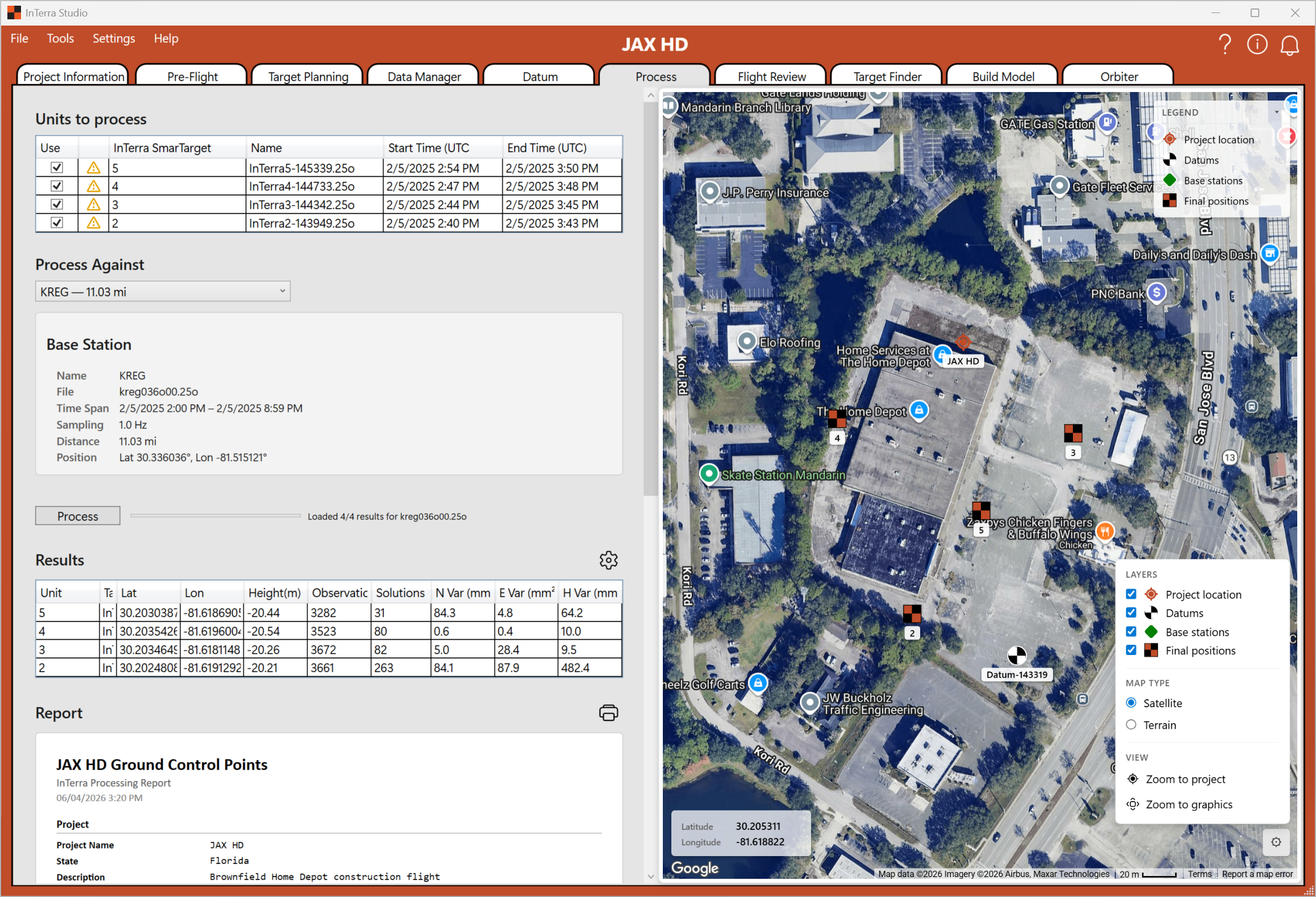
Screenshot: the Process tab with the units grid populated — the Use checkboxes, state icons, names, and status/cache columns.

What it's for. Select which surveyed units (your targets / points) to process against the base station, and run them.

When you use it. The final GNSS step — turning selected observations into corrected, final positions.

What you'll see. A units to process grid on the left and the map on the right.

• Target list. A table of your units with a Use checkbox, a state icon, the unit name, its status, and a cache indicator showing whether a result is current.
• Reprocess. Right-click a row that's up-to-date to reprocess that file specifically — handy when you change a setting and want to redo just one unit.
• Run. Process the selected units to produce their corrected positions.

Tips.

• Use the status column to see at a glance which units are done, pending, or need attention.
• Reprocess selectively rather than redoing everything when you only changed one input.

SmarTarget in the field

This section is the field reference for the physical SmarTarget hardware — how to deploy a unit on a survey, what the lights mean, and how to charge it. The software side — connecting units over USB, downloading the .ubx logs, and updating firmware — is covered under SmarTarget Manager above.

---

At a glance

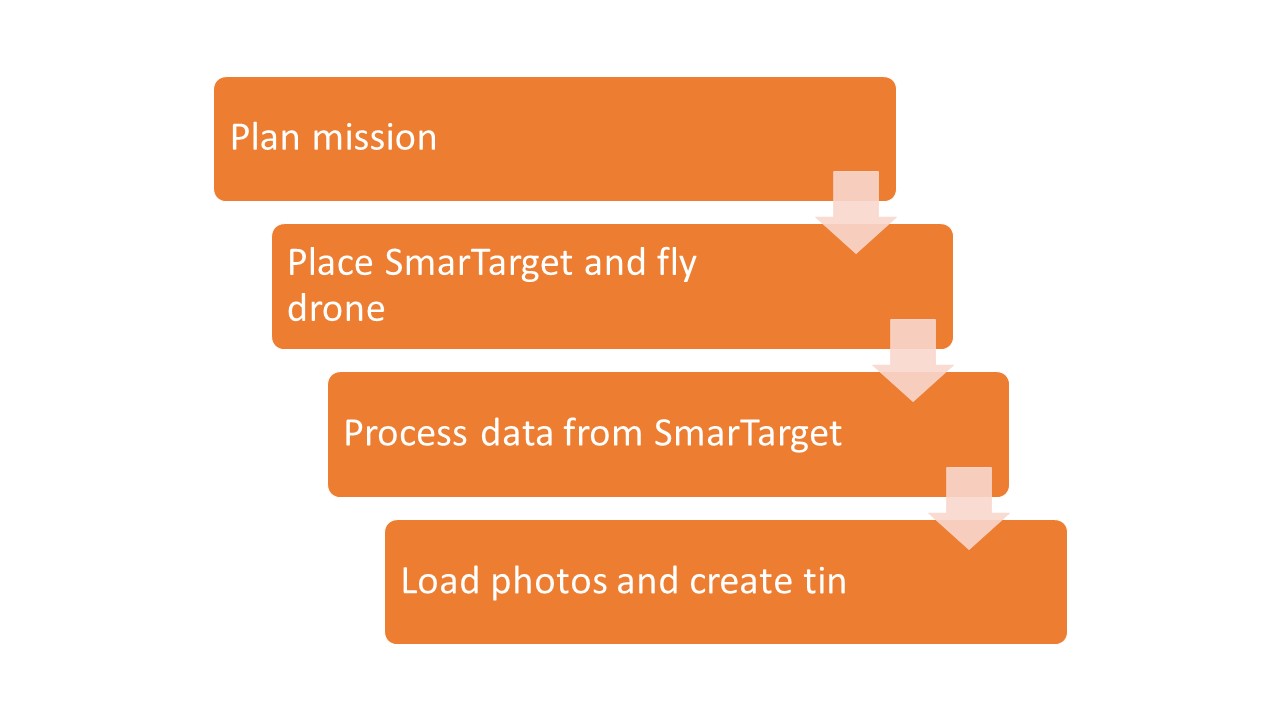
Mission flow: plan → place a SmarTarget on each target and fly → process the SmarTarget data → load the photos and build the model.

The typical field sequence with SmarTargets and a Datum unit is:

1. Set the Datum™ unit over your known location. Measure the height of the unit to the antenna line on the case (where the orange meets the black) and record it. Power the Datum on.
2. Lay out the cloth targets at your planned locations and stake them if the wind or surface needs it.
3. Power on a SmarTarget with its Power button and set it in the marked center placement zone of a cloth target. Repeat for each target.
4. Fly the mission.
5. Power off each SmarTarget and pick it up. Then turn off and retrieve the Datum unit.
6. Download the data from each unit over USB in SmarTarget Manager (let units recharge if needed).
7. Process the units in the Studio's GNSS workflow (Data Manager → Datum → Process).

Field tip — power the unit on and off while it's on the ground. First and last observations get tossed during processing if the unit looks like it's moving, so powering on or off while you're walking with it just throws away the first or last few seconds of good data.

---

The cloth targets

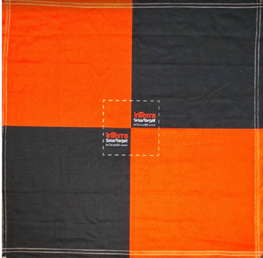
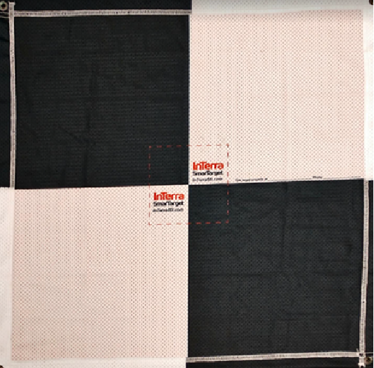
The two cloth target faces. The orange/black side reads strongly against concrete and asphalt; the white/black side reads strongly against grass and natural terrain.

Each SmarTarget ground marker is a reversible cloth target — orange/black on one side, white/black on the other — so you can pick the contrast that pops best against the surface you're flying over:

• White/black — best on grass, dirt, and most natural terrain.
• Orange/black — best on concrete, asphalt, and other light or grey built surfaces.

The cloth has reinforced grommets at each corner for staking or anchoring in wind, a clearly marked center placement zone for the powered-on SmarTarget, and a patch where you can write a contact name and phone number in case the target needs to be recovered or identified on site.

---

Reading the LEDs

The SmarTarget's LED panel — three indicators that together tell you everything about the unit's state.

Each SmarTarget has three indicator LEDs on the case, from left to right:

• Blue — Recording. Off until the unit is actively logging, then it blips briefly once per second as each batch of observations is written to memory. (The blip is short — about 10 ms — so look for a flicker, not a blink.)
• Green — GNSS. Slow glow while the unit is searching for satellites. Goes steady on once it has a fix. If it isn't lighting up at all, check for trees, buildings, or other overhead obstructions.
• Yellow — Power / Charge. On while the unit is charging over USB, off when the battery is full or the unit isn't plugged in.

The full state table — what each combination looks like, and what to do. The preview column shows a live mini-strip animated at the same frequencies the firmware uses, so you can match what you're seeing in your hand to the row.

Recording GNSS Power

State	Light pattern	What it means
Charging		Battery is topping up over USB. Yellow turns off when the unit is full.
Start-Up		Booting. Green and Blue alternate at 2 Hz (green leads) for about three seconds while the unit initializes.
Searching		Looking for a GNSS fix. Green ramps up and down slowly (~1.7 s per cycle) until it locks, then snaps to steady on.
Logging		Locked and recording. This is what you want to see in the field. Green steady on, Blue blips once a second.
Battery Low		Battery is too low to keep logging. The unit fades Blue + Green together for a few cycles and then shuts itself down. Charge it.
Fault Detected		Fault. Blue + Green flash together at 2 Hz. What to try: power cycle the unit, let the battery fully charge, then retry. If the fault persists, send the unit back to the factory.

When connected to a PC

Plug a SmarTarget into a PC over USB and the LEDs stop describing the field state and start describing the USB session instead — the unit deliberately won't log while connected, so Blue and Green are reused as "connected and ready" / "busy with a command" indicators. Yellow keeps following the charging circuit.

Yellow on every row below. The Yellow LED just follows the charging circuit: on while the unit is topping up, off when the battery is full. It's not part of the active pattern in any connected state, so the previews all show it on (the "plugged into a powered hub" case). Don't read anything else into yellow in this table.

State	Light pattern	What it means
Connected, idle		Unit is on USB and ready for the next command from SmarTarget Manager. Blue stays solid on between commands.
Listing files		Brief — both lights come on while the unit reads the SD card directory in response to a Ping / refresh from Manager.
Downloading a file		Blue and Green alternate while bytes are flowing — blue, then green, then blue — back and forth at a few times per second. The rate scales with how fast your USB port is moving the data, so on a slow port the alternation is slower.
Download complete		When the file finishes transferring, both Blue and Green flash together three times as a "done" chirp, then the unit drops back to the idle pattern (blue solid on).
Deleting a file		No visible LED change — the SD-card delete completes in a few milliseconds and the unit drops back to the idle pattern.

If you see the field-mode patterns (slow green glow, blue blip, etc.) while the unit is plugged in, something's off — power-cycle the unit and re-plug it.

---

Battery and charging

The powered 7-port USB charging hub, plugged into a wall outlet and charging several SmarTargets at once.

Each SmarTarget runs on a built-in 3.7 V, 2000 mAh Li-Polymer battery that's good for hundreds of charge cycles over the life of the unit. A full charge gives you more than 12 hours of runtime — well over a typical survey day.

• Use the powered USB hub that ships with the SmarTarget Kit. It has seven ports, can charge five SmarTargets at once, and has spare ports for phones or other USB devices.
• The hub must be plugged into a wall outlet to charge. A PC-to-hub USB connection alone won't charge the units — there isn't enough power. Plug the hub's wall adapter into a standard outlet.
• USB connection disables logging. When a unit is plugged in over USB, it will not turn on the GPS or write data to memory. That means you can safely manage files in SmarTarget Manager without the unit trying to record at the same time.
• Battery drains slowly even when idle — that's normal. All rechargeable batteries leak a small amount while sitting (it's called quiescent current). A SmarTarget will show some drop after weeks on the shelf, but at idle rates it would take roughly three years to drain a full battery.

---

In the office: file download and firmware

For pulling the raw .ubx GNSS logs off your units, checking battery state on each connected unit, and pushing firmware updates, see SmarTarget Manager above. Manager is the only place those operations happen in the Studio.

Modeler tabs

The Modeler tabs are where your photos become a model: you review flight quality and trim redundant images, pinpoint ground-control points in the imagery, then choose your outputs and build the model in the cloud.

Flight Review

Screenshot: the Flight Review tab — the photo viewer and map on top, the photo list (with the Keep / Outside / Redundant / Used flags) and the coverage-statistics card along the bottom.

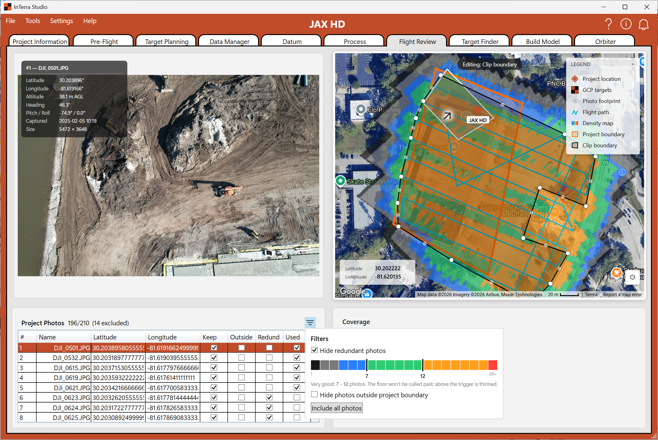
Screenshot: (optional detail) the filter popup open, showing the redundancy / boundary / coverage-band controls.

What it's for. Assess the overall quality and coverage of your flight, and cull redundant photos so you process only the images you actually need — saving processing time and cost without sacrificing coverage.

When you use it. After loading a flight's photos, before building the model.

What you'll see. The tab is split: a photo viewer and a map across the top, and a photo list plus a coverage statistics card along the bottom.

• Photo list. Every photo in the flight, with columns including the photo number and name, its latitude/longitude, and a set of flags: Keep (will this photo be used), Outside (is it outside your boundary), Redundant (is it duplicating coverage already provided by others), and Used (its final include state).
• Coverage statistics. A card summarizing the flight: average GSD, image size, total pixels, and the areas involved — how much ground your photos cover versus the area you'll actually model after clipping to the boundary.
• Filtering and culling. A filter popup lets you trim the set by redundancy, by the boundary, and along a coverage band slider, so you can dial coverage down to what's needed and drop the rest. The map and statistics update so you can see the effect of your choices.
• Ground-control progress. If you've loaded ground-control points, Flight Review shows your tagging progress so you know how much GCP work remains.

Tips.

• Culling is about removing redundancy, not coverage — InTerra's coverage view helps you keep enough overlap everywhere while dropping the photos that only repeat what neighbors already capture.
• Check the Outside flag to drop photos shot well beyond your site that add processing cost without adding value.
• Watch the modeled area versus photo coverage area in the statistics to understand how much your boundary clip is trimming.

Target Finder

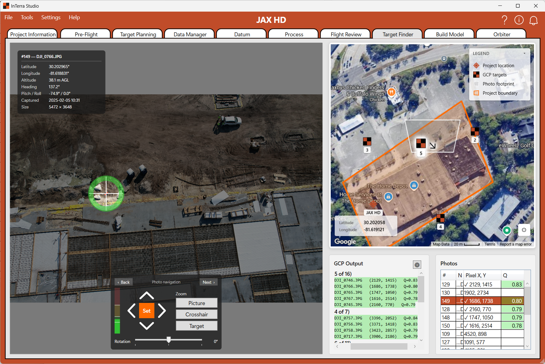
Screenshot: the Target Finder tab — the large image viewer with the crosshair mask over a target on the left, the map top-right, and the GCP tree beside the photo grid bottom-right.

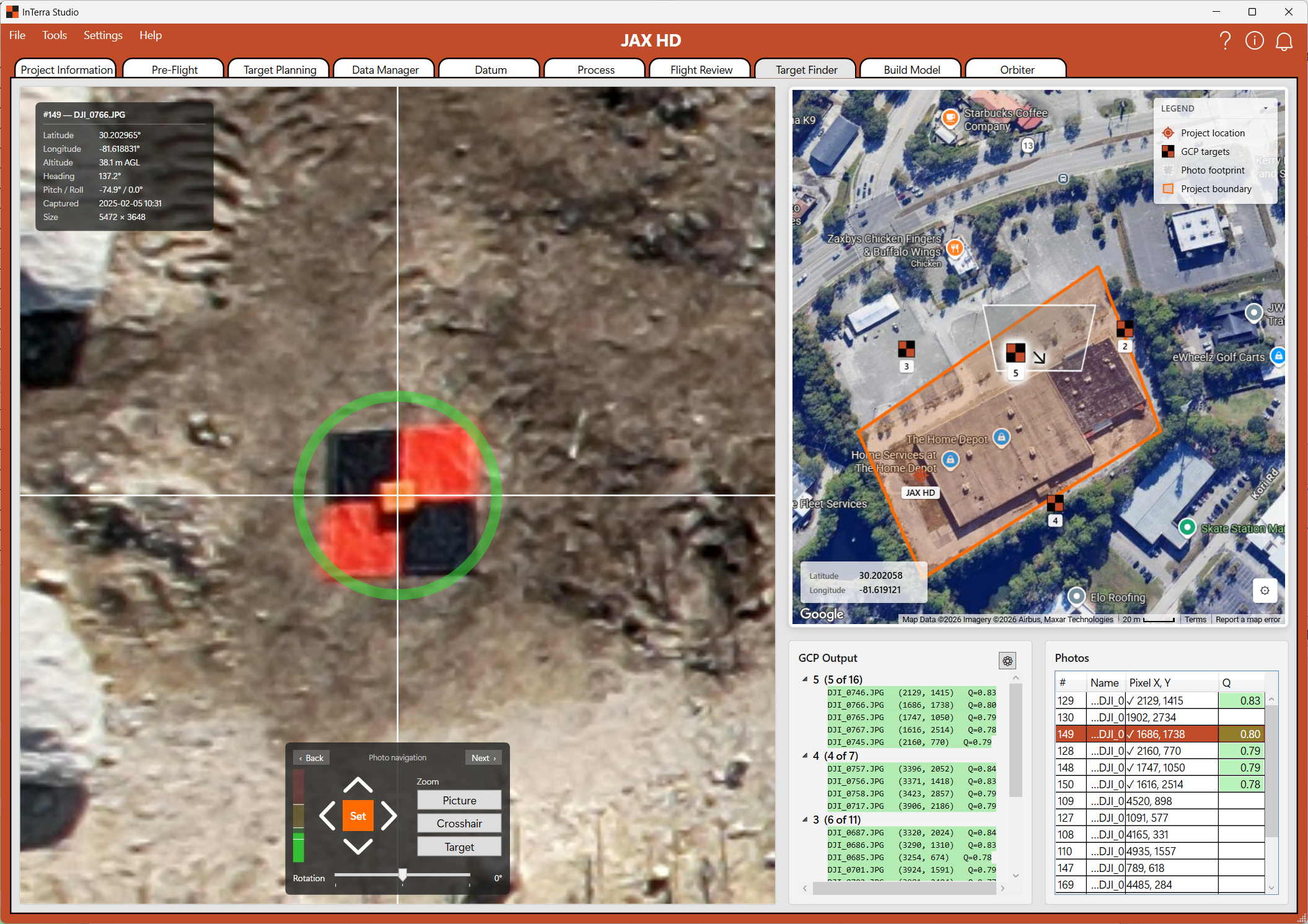
Screenshot: (detail) a zoomed-in view of the crosshair mask centered on a ground target.

What it's for. Pinpoint exactly where each ground-control point (GCP) appears in your photos — to the pixel — so the model can be georeferenced accurately against your surveyed control.

When you use it. After Flight Review, once you've loaded ground control — this is the careful, per-point tagging work that drives final accuracy.

What you'll see. A large image viewer on the left (most of the tab), a map at the top-right, and at the bottom-right a GCP tree beside a photo grid.

• Image viewer with crosshair mask. The viewer overlays a crosshair "mask" centered on where InTerra predicts the GCP sits in the current photo. You fine-tune the exact pixel. The mask can be rotated (roughly -45° to +45°) to line up with the target, and you can adjust its size.
• Photo navigation. Move Back/Next through the candidate photos for a given GCP; your zoom is preserved so you stay locked in on the target as you step through images.
• Nudge and set. Use the D-pad nudge controls to move the crosshair a pixel at a time, then Set Target to confirm the GCP's location in that photo.
• Zoom presets. Quick zoom buttons (for example, frame the whole picture, zoom to the crosshair, or zoom to the target) so you can jump between context and precision.
• GCP tree. Your control points and the photo picks you've confirmed for each, color-coded by match quality — green for strong agreement, yellow and red for picks worth re-checking. A settings popup lets you toggle per-target colors and filter which quality rows you see.
• Photo grid. For each candidate photo, the predicted pixel X,Y of the GCP and a quality (Q-tier) score, so you can prioritize the photos most worth tagging.

Tips.

• Tag each GCP in several well-spread photos for a strong, well-constrained solution.
• Let the color tiers guide you — green picks are agreeing; revisit yellow and red, which are where small mistakes hide.
• Use the nudge controls for the final pixel or two rather than trying to click perfectly; precision here pays off directly in your residuals.

Build Model

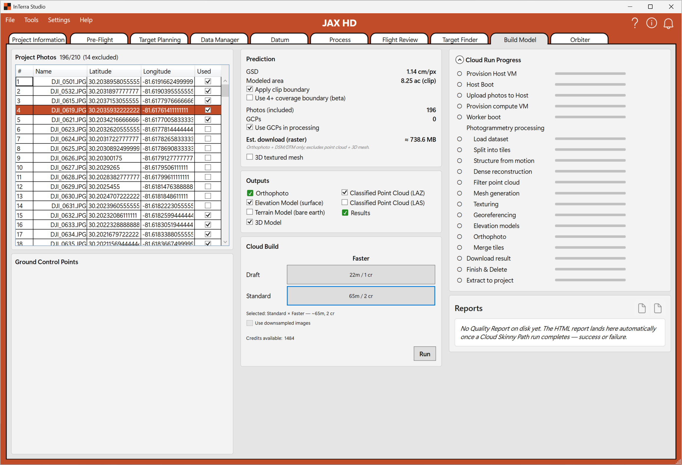
Screenshot: the Build Model tab — the photos and ground-control columns on the left, and the Prediction card, Outputs checkboxes, and the cloud-build control in the middle.

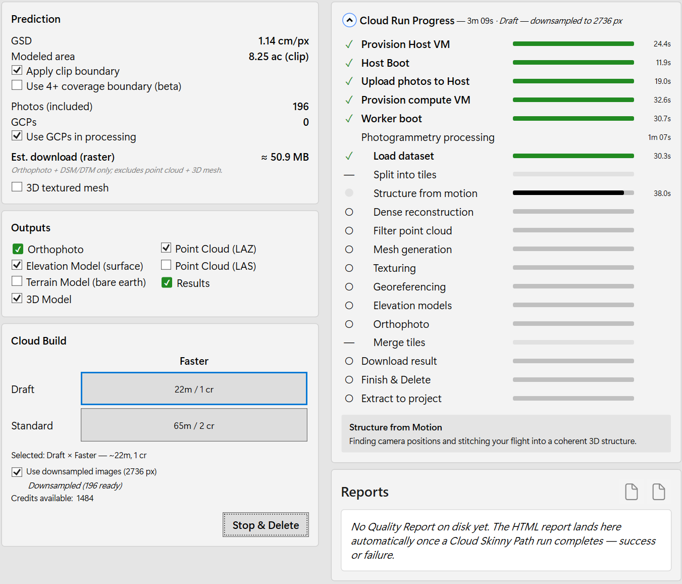
Screenshot: (detail) a close-up of the Prediction card (GSD, modeled area, counts, estimated credits, download size) and the Outputs list.

What it's for. The launch pad for cloud photogrammetry: a final review of the photos and ground control going in, a prediction of what you'll get, your choice of outputs, and the button that starts the cloud build.

When you use it. Last in the imagery workflow — when you're ready to turn your reviewed photos and tagged control into deliverables.

What you'll see. Three columns: your photos and ground-control points on the left (a read-only mirror of your Flight Review and Target Finder work), a middle column with Prediction, Outputs, and the cloud-build control, and supporting detail.

• Project Photos & Ground Control. A final, read-only look at exactly which photos will be processed (with their Used state) and which GCPs will anchor the model — so you can confirm the inputs before you spend processing time.
• Prediction. Before you commit, InTerra estimates the job: the resulting GSD, the modeled area, the photo count and GCP count, whether the model will be clipped to your boundary and/or limited to the coverage boundary, and an estimated download size for the results. This is your sanity check that the run will produce what you expect.
• Outputs. Choose your deliverables:
• Orthophoto — the georeferenced, stitched top-down image (always produced).
• Elevation Model (DSM) — a surface model including everything on the ground (buildings, vegetation, structures).
• Terrain Model (DTM) — a bare-earth model with above-ground objects removed.
• 3D Model — the textured mesh you can spin in Orbiter.
• Point Cloud (LAZ/LAS) — the dense 3D point set for CAD/survey software.
• Quality Results — the client-facing results report summarizing accuracy and deliverables (and carrying your branding).
• Start the cloud build. Kick off processing. From here your inputs are sent to the dedicated, encrypted, per-job processing — InTerra's Zero Persistence Computing — described under Explanation → Zero Persistence Computing, and InTerra reports progress as the model is built.

Tips.

• Only choose the outputs you actually need — each one adds processing time and cost. You can always run again for more.
• Use the Prediction numbers to catch surprises (an unexpectedly huge modeled area, or a download size that won't fit your connection) before you start.
• Turn on clip to boundary to get clean deliverables limited to your site rather than ragged edges spilling past it.

Cloud builds: options, credits, and progress

Processing options. When you start a build you choose a processing option that trades speed against completeness:

• Draft — a faster, lighter pass for a quick look at coverage and the orthophoto. Great for checking a flight worked before committing to the full job.
• Standard — the full-quality build that produces your final deliverables.

The option is paired with a processing-machine choice, shown in plain terms (for example, the machine's processor and memory) so you can see the horsepower behind each option rather than opaque codes.

Credits. Cloud builds consume credits from your account. The Build Model → Prediction card shows an estimated credit cost for the run before you start, and your current credit balance is always visible under Help → About. Larger jobs (more photos, more area, finer GSD) and faster machines use more credits — which is exactly why Flight Review culling and choosing only the outputs you need save real money, not just time. If you don't have enough credits for a run, InTerra tells you up front (and through the notification center) rather than failing partway.

Progress. Once a build starts, InTerra reports live progress as the job moves through its stages, so you can see it's working and roughly how far along it is. You don't need to keep the build window in focus.

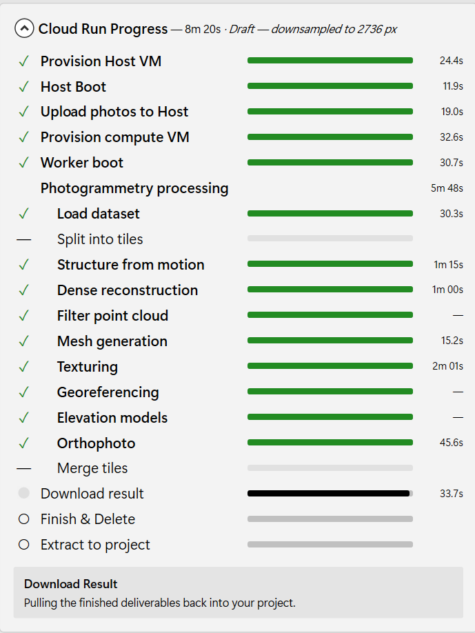
Screenshot: a build in progress, showing the live stage/progress display so readers know what a running job looks like.

Reconnecting to a running build. Cloud builds can take a while, and you don't have to babysit them. If you close InTerra, lose your connection, or your computer sleeps while a build is running, InTerra remembers the active job. When you reopen the project it can reconnect to the still-running build and pick up where it left off — you won't lose the job or pay for it twice. This pairs with the dedicated-machine design described under Explanation → Zero Persistence Computing: the job keeps running on its own private machine whether or not your app is watching.

Your reports

InTerra produces two kinds of report, aimed at two different audiences.

• Results report (client-facing) — the polished summary you hand to your client: project details, deliverables, accuracy (including per-control-point residuals when you used ground control), coverage, and preview imagery. This is the Quality Results output you select on Build Model, and it carries the branding you set under Settings → Branding… so it looks like your company's deliverable.
• Processing report (operator-focused) — a behind-the-scenes record of the run for you: what you sent, what came back, how long each stage took, and the settings used. It's the engineer's-eye view for understanding and tuning a run, not for sharing with clients.

Both reports are generated as self-contained files you can open in a browser, and you can save them as PDF for emailing or archiving. The Results report, in particular, is designed to print cleanly so it reads like a finished deliverable.

Orbiter

Orbiter is InTerra's interactive viewer for finished deliverables — pan and zoom the orthophoto in 2D, orbit the 3D mesh or point cloud, mark up and measure the site, and export your contours and drawings to CAD.

The Orbiter viewer (2D & 3D)

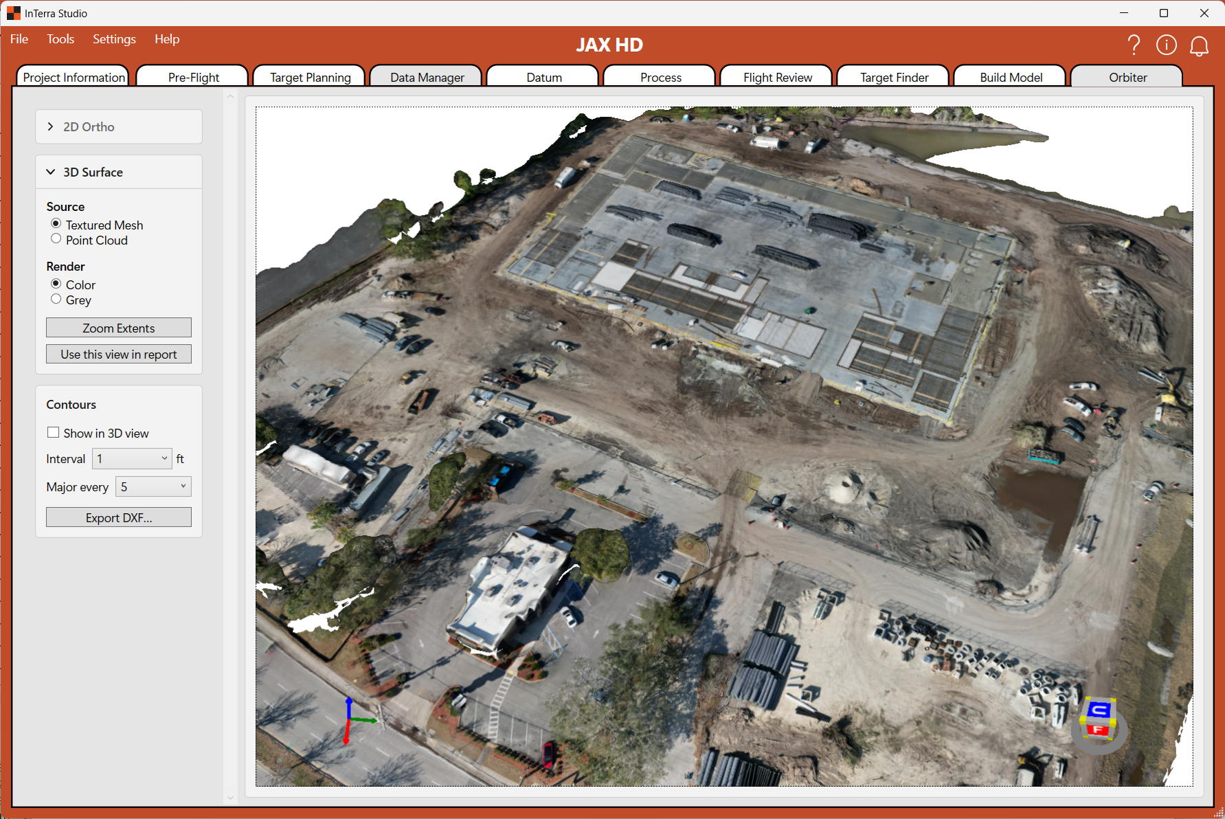
Screenshot: the Orbiter tab in 3D, showing the textured mesh (or point cloud) with the tools panel on the left and the view cube / axes visible.

Screenshot: Orbiter in 2D, showing the zoomable orthophoto.

What it's for. Explore your finished deliverables interactively — pan and zoom the orthophoto in 2D, and orbit the 3D mesh or point cloud — so you can inspect the model, measure it, and show it to clients.

When you use it. After a build completes, to review and present results.

What you'll see. A tools panel on the left and a large viewer on the right that switches between a 2D map view (orthophoto) and a 3D view (mesh or point cloud), with an on-screen view cube and coordinate axes (oriented Z-up).

• Source selector. Switch what you're looking at:
• Orthophoto — the 2D, zoomable, pannable top-down image.
• Mesh — the textured 3D surface model.
• Point Cloud — the dense 3D point set.
• Contours. In 3D, toggle contour lines (with distinct minor and major lines) drawn across the surface to read elevation at a glance.
• Measurement and markup. Place points, draw lines, and outline polygons on the orthophoto, with editable colors, names, and computed length / area / volume — see Drawing on the 2D viewer below.
• Zoom Extents. Frame the whole site in one click when you've zoomed or orbited away.

Tips.

• Use the view cube to snap to top/front/side views quickly.
• A large point cloud can take a moment to load — a loading indicator appears while it decodes; let it finish before interacting.
• Switch between the orthophoto and 3D views to answer different questions: the ortho is best for plan-view position and measurement, the 3D views for shape, volume, and structure.

Drawing on the 2D viewer

Screenshot: the draw toolbar in the 2D view, showing the Point, Line, and Polygon buttons with their color swatches.

The 2D (orthophoto) view has a built-in drawing layer for marking up your site — place points, draw lines, and outline polygons directly on the ortho. Each element is saved with the project (in Viewer/orbiter.json) and comes back exactly as you left it the next time you open it.

The three element types share one Feature List in the left panel, grouped into Points, Lines, and Polygons layers. Each layer has its own visibility toggle so you can hide or show a whole class of elements at once without deleting anything.

Drawing an element. Pick the element type from the toolbar — Point, Line, or Polygon — and the cursor arms for drawing:

• Point. Click once on the ortho. The point is committed immediately and selected so you can name it and set its color.
• Line. Click each vertex along the path. A rubber-band preview follows the cursor from the last vertex. Finish with Enter or a double-click (minimum two vertices).
• Polygon. Click each vertex around the shape. Finish with Enter or a double-click to close the ring (minimum three vertices — don't repeat the first vertex; it closes automatically).

While you're drawing a line or polygon, Backspace removes the last vertex you placed (useful for a misclick), and Esc cancels the in-progress draw entirely.

Editing an element. Click an element on the map, or its row in the Feature List, to select it. A selected element shows its vertices as drag handles — drag a handle to move that vertex, or drag a single-vertex point itself to relocate it. Insert or remove a vertex on a line or polygon via the mid-segment handles that appear between existing vertices. Click an empty area of the map to deselect. Edits save automatically with the project.

Erasing an element. Select it, then press Delete, or use the delete button next to its row in the Feature List. There is no undo for a delete — re-draw the element if you need it back. To hide a whole class of elements without deleting, toggle the Points / Lines / Polygons layer visibility in the Feature List instead.

The Properties card. Selecting any element opens a Properties card with editable fields and computed readouts.

Screenshot: the Properties card for a selected Point, showing name, color, and the lat / lon / grid / elevation readout.

Screenshot: the Properties card for a selected Line, showing name, color, line style, total length, and the per-segment length / slope table.

Screenshot: the Properties card for a selected Polygon, showing name, color, line style, fill opacity, perimeter, area, the per-vertex / per-segment table, and the Volume section.

The editable fields are the same for every element type:

• Name — what the element is called in the Feature List and on any exported snapshot.
• Color — set per element, so you can color-code by meaning (e.g. boundary vs. obstruction vs. stockpile).
• Line style (lines and polygons) — solid, dashed, or dotted stroke.
• Fill opacity (polygons only) — how transparent the polygon fill is so the ortho underneath stays readable.

What the card shows depends on geometry:

• Point — latitude / longitude (WGS 84), grid coordinates in the project's coordinate system, and the elevation sampled from the DSM or DTM at that pixel.
• Line — total length, plus a per-segment table with each segment's length and slope (%).
• Polygon — perimeter and enclosed area, the elevation at each vertex, a per-segment table, and — when an elevation surface is loaded — the Volume section described below.

Lengths and areas are formatted in your chosen units (metric or imperial).

Volumes — stockpiles, holes, and ditches (polygons). When you draw a polygon over an area that has elevation coverage, the Properties card gains a Volume section that computes a cut/fill volume against a chosen base surface. The same tool works for piles (how much material sits above the ground — e.g. a stockpile) and for excavations like holes, pits, and ditches (how much material it would take to fill them in):

• Source surface — DSM (top-of-pile, including vegetation and structures) or DTM (bare-earth where one was generated).
• Base — choose how the reference surface under the pile is defined:
  • Average of surface — the mean elevation of all cells inside the polygon. Quick and stable; reads the pile as if it sat on a flat pad at the inside average.
  • Lowest point — the lowest cell elevation inside the polygon. Conservative for cut/fill — treats the deepest spot in the footprint as ground.
  • Best-fit plane — a tilted least-squares plane through the perimeter-vertex elevations. Follows a uniformly-sloped pad (ramp, graded surface) instead of forcing a flat base. With this mode the base has no single number, so the custom-elevation field is hidden.
  • Custom — type in a fixed elevation. Typing a value into the base field also switches the mode to Custom automatically.
• Readout — Fill (material above the base), Cut (void below the base), and Net (Fill − Cut, positive for a net pile and negative for a net excavation). Reported in cubic metres for metric projects, cubic yards for imperial-unit projects (the standard US earthworks quantity unit). Also shows the cell count the computation summed over.

To use it for a stockpile: outline the toe of the pile (where the slope meets the ground), pick the source surface (DSM for the whole pile, DTM for only what's above bare earth), and pick the base mode that best matches the surrounding pad. The Fill value is the pile's rough volume.

To use it for a hole, ditch, or other excavation: outline the rim where the ground starts to drop, pick the source surface (DSM is usually right — it follows the dirt at the bottom of the pit), and pick a base mode that represents the surrounding finished grade. The Cut value — the void below the base — is the rough volume of material it would take to fill the feature up to that grade.

The card updates live as you adjust the base.

A few practical notes:

• The accuracy of the volume is dominated by the base surface choice, not the cell math — picking the right base mode for the site matters more than which source raster you pick.
• Works well for normal piles on roughly flat or uniformly-sloped ground. For piles on heavily uneven pads with multiple break-elevations, place the polygon along a section where the ground is most uniform, or pick Best-fit plane so a tilt is allowed.
• Outline the rim of the feature — the toe of a pile, or the lip of a hole — not the top of a pile or the bottom of a pit. The volume between your ring and the surface inside it is what's reported: the material above the base for piles (read Fill), the void below the base for excavations (read Cut).

Exporting contours and drawings to CAD (DXF)

The Export DXF button (in Orbiter's 3D contour tools) writes a single DXF file you can open in any CAD package — AutoCAD, Civil 3D, MicroStation, and so on. It captures both of Orbiter's vector outputs in one file:

• the generated contour lines (on CONTOUR_MAJOR / CONTOUR_MINOR layers), and
• every point, line, and polygon you drew on the orthophoto.

Each drawn element is placed on its own CAD layer, named after the element. So the Name you give a feature in the Properties Card becomes its DXF layer name — name your elements deliberately (e.g. Boundary, Stockpile-3, Drainage) and they arrive in CAD already organized by layer, in the element's color. Points export as DXF points, lines as open polylines, and polygons as closed polylines.

All coordinates are written in the project's Grid coordinate system — the same CRS as the rest of your deliverables — so the drawing lands at true 1:1 scale and overlays your other survey data without shifting.

Clicking Export DXF writes the file immediately; there's no dialog. It's saved into the project's Reports folder as {project}.dxf. The button is available whenever there are contours or drawn elements to export — re-click it after adding more contours or drawings to refresh the file.

How the tabs connect

The tabs aren't independent screens; each one's work flows into the next. Seeing the chain helps you understand why order matters and where a change ripples.

• Project Information is the root. Your location, boundary, and coordinate system feed everything downstream: the map basemap, photo footprints, coverage statistics, the area that gets modeled, how outputs are clipped, and the header on your client report. Change the boundary or CRS and you affect the whole job.
• Pre-Flight sets your expectation for GSD and footprint, which is the yardstick you compare against on Flight Review and Build Model.
• Target Planning defines the physical targets you'll place — the same targets you later pinpoint in Target Finder, and whose surveyed positions become your ground control.
• Data Manager → Datum → Process form a chain: imported GNSS logs feed the base-station reference, which feeds the processing that produces corrected positions — your survey-grade ground control.
• Flight Review decides which photos are "Used". That culled set is exactly what Build Model sends to the cloud — so culling here directly shapes the cost and content of the build.
• Target Finder produces your confirmed GCP picks. Those drive how the model is georeferenced during the build and the accuracy figures (residuals) that appear in your Results report.
• Build Model gathers the used photos, the ground control, and your chosen outputs, and runs the cloud build. Its results flow two ways: into Orbiter for viewing and measuring, and into your reports.

Because the imagery tabs all read from one shared source of truth, what you do on Flight Review and Target Finder shows up consistently on Build Model — there's no need to re-enter anything; the tabs are different views of the same project data.

Map legend

Every map has a layer legend in its top-right corner listing the symbols in play on that tab, with a checkbox to show or hide each layer. Different tabs show different layers; this is the complete reference for every symbol you may see, grouped by purpose.

Symbol	Name	What it means
Project & area
	Project location	The map pin marking where the project sits, from the address or coordinates you set on Project Information.
	Project boundary	The outline of your survey / flight area — a rectangle or a buffered linear corridor.
	Boundary centerline	The editable centerline of a Linear (corridor) boundary; the corridor is buffered around it.
	Clip boundary	An optional polygon that limits cloud processing (ortho / DEM) to a sub-area, to cut cost on corridor jobs.
Flight planning
	Flight lines	The planned parallel passes the drone flies to cover the area.
	Flight path	The actual path flown, reconstructed from the captured photo positions.
	Camera positions	Where each photo was taken — one marker per exposure.
	Photo footprints	The ground area each photo covers; the overlap shows how redundant your coverage is.
	Coverage density	Photo-overlap heatmap (blue = thin, red = heavy) used to plan coverage and cull redundant photos. Shown as Planning density on the planning tabs and Density map in Modeler.
Ground control & reference
	Planned datum	The planned survey anchor point the targets are distributed around (round target, distinct from the square field targets).
	Targets (planned / GCP)	Square ground-control targets — planned positions to place in the field (Target Planning) and detected GCPs (Modeler). Orange or white, whichever contrasts better with the ground.
	Base stations	A GNSS base station location.
	CORS stations	Continuously Operating Reference Stations used to compute corrections for the datum.
	Datums (RTK)	RTK datum / monument points on the Data Manager map.
	NGS monuments	Published survey monuments. Shape = control type (triangle horizontal, circle vertical, square both); filled = adjusted, open = other quality. See the Locator tabs → NGS monuments overlay section for the full key.
Imagery & elevation
	Ortho photo	The stitched orthophoto overlay on the map.
	DSM (surface)	Digital Surface Model raster — the top of everything (vegetation, structures included).
	DTM (bare earth)	Digital Terrain Model raster — bare ground, with objects filtered out.
	Contours	Elevation contour lines — darker major lines, lighter minor lines.
Drawing (Orbiter)
	Points	Point annotations you draw on the orthophoto.
	Lines	Line annotations you draw (with measured length).
	Polygons	Polygon annotations you draw (with measured area and cut/fill volume).

The color of any individual drawn element (point, line, polygon) is set per-element in its Properties Card, so on the map your own annotations may differ from the default colors shown here.

Glossary

• AGL (Above Ground Level) — flight height measured from the ground beneath the drone, as opposed to height above sea level. The key input on Pre-Flight.
• Boundary — the polygon you draw on Project Information describing your site's extent. Drives modeled area, coverage stats, and output clipping.
• CRS (Coordinate Reference System) — the combination of datum and projection your project's coordinates are expressed in (for example, a state-plane or UTM zone). Set on Project Information.
• Credits — the units a cloud build consumes from your account. Your balance is shown under Help → About; an estimate for a run appears in Build Model → Prediction.
• Cull — removing redundant photos (on Flight Review) that only repeat coverage already provided by neighbors, to cut processing without losing coverage.
• Draft / Standard — the two cloud-build processing options. Draft is a fast, light pass for a quick look; Standard is the full-quality build for final deliverables.
• Datum — the reference surface/position your survey is measured against. In GNSS work it's also the base-station reference you select on the Datum tab.
• DSM (Digital Surface Model) — an elevation model that includes everything on the surface: buildings, vegetation, and structures.
• DTM (Digital Terrain Model) — a bare-earth elevation model with above-ground objects removed.
• Ellipsoidal height — height measured from a smooth mathematical model of the earth; what raw GNSS produces.
• GCP (Ground Control Point) — a physical, surveyed target on the ground whose precise position is known. Tagging GCPs in imagery (on Target Finder) georeferences and validates the model.
• GNSS (Global Navigation Satellite System) — the satellite positioning systems (GPS and others) your receiver logs; processed on the Data Manager / Datum / Process tabs.
• GSD (Ground Sample Distance) — the real-world size of one image pixel on the ground (e.g. 1.5 cm/px). Lower is finer detail. Computed on Pre-Flight, reported on Flight Review and Build Model.
• Orthometric height — height measured from the geoid (effectively "above mean sea level"); what most survey/engineering deliverables expect. Chosen on Project Information.
• Orthophoto — a georeferenced, distortion-corrected, stitched top-down image of the site. A core deliverable.
• Point cloud (LAS/LAZ) — a dense set of 3D points reconstructed from the imagery, used in CAD and survey software. LAZ is the compressed form.
• Processing report — the operator-focused, behind-the-scenes record of a cloud build (inputs, stage timings, settings). Contrast with the client-facing Results report.
• PPK — Post-Processed Kinematic: the correction technique Studio uses to derive precise positions for each SmarTarget (and the Datum) from their recorded GNSS observations and a reference receiver.
• Results report — the polished, client-facing summary of a job (the Quality Results output on Build Model), carrying your branding.
• RINEX — a standard exchange format for GNSS observation data, used for the base-station/datum reference on the Datum tab.
• SmarTarget — InTerra's ground-marker definitions (managed via Tools → SmarTarget Manager…) — the physical targets you place and detect in imagery.
• UBX — the raw log format produced by u-blox GNSS receivers, imported on the Data Manager tab.

Scaffolding page.